

"P-value nasıl hesaplanır?" sorusunun kısa cevabı: verinize uygun testi seçip test istatistiğini (t, z, χ² veya F) hesaplarsınız; ardından sıfır hipotezi doğruyken en az bu kadar uç bir istatistik elde etme olasılığını o istatistiğin dağılımından okursunuz. İki bağımsız grup için yazılım bu üç adımı tek çağrıda yapar: Python'da stats.ttest_ind(a, b, equal_var=False), Excel'de =T.TEST(aralık1;aralık2;2;3). Bu rehberde tek bir veri seti üzerinden p-değerini elle, Python'la ve Excel/Google E-Tablolar'la hesaplıyor; test seçimini, tek ve çift kuyruklu testleri, raporlamayı, varsayımları, çoklu karşılaştırmayı ve yorum hatalarını aynı örnek üzerinden ele alıyoruz. Bütün sayılar SciPy ve statsmodels ile doğrulandı.
1. P-değeri nedir? Sezgi ve doğru tanım
Her hipotez testi şu soruyla başlar: Gerçekte hiçbir fark olmasaydı, yalnızca örneklemenin rastlantısallığı yüzünden en az bu kadar büyük bir fark ne sıklıkla görülürdü? "Fark yok" varsayımı sıfır hipotezidir (null hypothesis, H0); sınanan iddia ise alternatif hipotezdir (H1).Tanım: p-değeri (p-value), H0 doğruysa ve testin varsayımları (bağımsız gözlemler, uygun dağılım modeli) sağlanıyorsa, en az gözlenen kadar uç bir test istatistiği (t, z, χ² veya F) elde etme olasılığıdır. Küçük bir p, verinin "H0 + varsayımlar" modeliyle uyuşmadığını söyler; fazlasını değil.
- Anlamlılık düzeyi (significance level, α): Veriye bakmadan önce seçilen eşik; p ≤ α ise H0 reddedilir. α, doğru bir H0'ı reddetme (I. tip hata) olasılığıdır.
- Serbestlik derecesi (degrees of freedom, df): t, χ² ve F dağılımlarının biçimini belirleyen parametre; kabaca varyans tahminine giren bağımsız bilgi miktarı. df küçüldükçe t dağılımının kuyrukları kalınlaşır.
- Tek ve çift kuyruk: p'nin dağılımın bir ucundan mı (one-tailed), iki ucundan mı (two-tailed) hesaplandığı. Türkçe kaynaklarda tek yönlü ve çift yönlü test diye de geçer.
2. Örnek veri seti: iki tedarikçinin filamenti
Bir atölye, iki tedarikçiden aldığı PLA filamentle aynı ayarlarda ve rastgele sırayla çekme numuneleri (tensile test bar) basıp çekme dayanımlarını (MPa) ölçüyor. Değerler öğretim amacıyla kurgulanmıştır.| Grup | Ölçümler (MPa) | n | Ortalama | Standart sapma |
|---|---|---|---|---|
| Tedarikçi A | 53, 45, 55, 50, 58, 52, 49, 54 | 8 | 52,0 | 4,0 |
| Tedarikçi B | 47, 50, 46, 48, 51, 45, 49, 48, 50, 46 | 10 | 48,0 | 2,0 |
Hipotezler: H0: μA = μB, H1: μA ≠ μB (çift kuyruklu); α = 0,05 analizden önce sabitlendi. A grubu hem daha küçük hem de daha dağınık; bu ayrıntı sonucu belirgin biçimde etkileyecek.
3. Doğru testi seçmek: karar tablosu
Testi veri tipi (ölçüm mü, sayım mı), grup sayısı ve ölçümlerin eşleştirilmiş olup olmadığı belirler.| Soru ve veri | Parametrik test | Parametrik olmayan alternatif | Python |
|---|---|---|---|
| Tek grubun ortalaması bir hedef değerden (ör. 50 MPa) farklı mı? | Tek örneklem t-testi | Wilcoxon işaretli sıralar testi | stats.ttest_1samp |
| İki bağımsız grubun ortalaması farklı mı? | Welch t-testi (eşit varyans varsayılırsa Student) | Mann–Whitney U | stats.ttest_ind(a, b, equal_var=False) |
| Aynı parçalarda önce/sonra ölçümü | Eşleştirilmiş t-testi | Wilcoxon işaretli sıralar testi | stats.ttest_rel |
| Üç veya daha fazla bağımsız grup | Tek yönlü ANOVA + Tukey HSD gibi bir post-hoc test | Kruskal–Wallis | stats.f_oneway; varyanslar farklıysa statsmodels anova_oneway(use_var="unequal") |
| İki kategorik değişken (sayımlar) | Ki-kare bağımsızlık testi | Fisher kesin testi (beklenen sayılar küçükse) | stats.chi2_contingency, stats.fisher_exact |
| Popülasyon standart sapması gerçekten biliniyor ya da büyük örneklemde oran | z-testi | Kesin binom testi | stats.binomtest, statsmodels proportions_ztest |
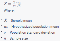
Sık yapılan iki hata var. Birincisi, z-testi "n > 30 ise kullanılan test" değildir: standart sapma örneklemden tahmin ediliyorsa doğru referans dağılımı t dağılımıdır ve t, n büyüdükçe zaten normal dağılıma yaklaşır. Örnek verimize statsmodels kütüphanesindeki ztest(a, b) uygulanırsa p ≈ 0,006 çıkar: doğru Welch sonucunun (0,028) beşte biri. İkincisi, Mann–Whitney U ortalamaları karşılaştırmaz; bir gruptaki değerlerin diğer gruptakilerden büyük olma eğiliminde olup olmadığını sınar. Sonucu medyan karşılaştırması gibi okumak ancak iki dağılımın biçimi aynıysa doğrudur.
4. Elle hesaplama: t istatistiği, serbestlik derecesi ve p
Gruplar bağımsız ve yayılımları belirgin biçimde farklı olduğu için Welch t-testini adım adım uyguluyoruz.Adım 1: Ortalamalar ve varyanslar
Kod:
A: toplam = 416, n = 8   →  ortalama = 52,0
   ortalamadan sapmalar: 1, -7, 3, -2, 6, 0, -3, 2
   kareler toplamı = 1+49+9+4+36+0+9+4 = 112  →  s² = 112/7 = 16,0  (s = 4,0)

B: toplam = 480, n = 10  →  ortalama = 48,0
   ortalamadan sapmalar: -1, 2, -2, 0, 3, -3, 1, 0, 2, -2
kareler toplamı = 1+4+4+0+9+9+1+0+4+4 = 36 → s² = 36/9 = 4,0 (s = 2,0)Adım 2: Standart hata ve t
Kod:
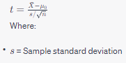
SE = √(sA²/nA + sB²/nB) = √(16/8 + 4/10) = √(2,0 + 0,4) = √2,4 = 1,549
t  = (52,0 − 48,0) / 1,549 = 2,582
Adım 3: Welch–Satterthwaite serbestlik derecesi
Kod:
df = (sA²/nA + sB²/nB)² / [ (sA²/nA)²/(nA−1) + (sB²/nB)²/(nB−1) ]
   = 2,4² / [ 2,0²/7 + 0,4²/9 ]
= 5,76 / (0,5714 + 0,0178) = 5,76 / 0,5892 = 9,78Adım 4: t'den çift kuyruklu p'ye
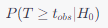
P-değeri, t(9,78) dağılımında ±2,582'nin dışında kalan iki kuyruktaki alanların toplamıdır: p = 2 × P(T ≥ 2,582). Elle çalışırken p'yi t tablosundan bir aralık olarak okursunuz; kesirli df için temkinli yol, bir alttaki tamsayıyı (9) kullanmaktır:
Kod:
df = 9 için çift kuyruklu kritik değerler:
  p = 0,05  →  2,262
  p = 0,02  →  2,821
2,262 < 2,582 < 2,821   →   0,02 < p < 0,05
Kod:
t² = 16 / 2,4 = 6,667
x  = df / (df + t²) = 9,776 / (9,776 + 6,667) = 0,5945
p = I_x(df/2; 1/2) = I_0,5945(4,888; 0,5) = 0,0278Karşılaştırma: Student t-testi
Eşit varyans varsayan Student testi iki grubun varyansını birleştirir (birleştirilmiş varyans, pooled variance): sp² = (7·16 + 9·4)/16 = 9,25, SE = √(9,25 · (1/8 + 1/10)) = 1,443, t = 2,773, df = 16, p = 0,0136. Bu, Welch p'sinin yaklaşık yarısıdır: birleştirme, büyük ve az dağınık B grubuna fazla ağırlık verip A'nın dağınıklığını gizler ve standart hatayı küçültür. Daha dağınık olan büyük grup olsaydı hata ters yönde olurdu: Student testi gereğinden temkinli kalırdı. t yerine normal dağılım kullanılsaydı p ≈ 0,0098 çıkardı: küçük df'de kalın kuyrukları yok saymak p'yi yaklaşık üçte birine indirir.5. Python ile: SciPy ve statsmodels
Python:
import numpy as np
from scipy import stats

a = np.array([53, 45, 55, 50, 58, 52, 49, 54])          # Tedarikçi A
b = np.array([47, 50, 46, 48, 51, 45, 49, 48, 50, 46])  # Tedarikçi B

welch = stats.ttest_ind(a, b, equal_var=False)
print(welch.statistic, welch.df, welch.pvalue)   # 2.582  9.776  0.0278
print(welch.confidence_interval(0.95))           # low=0.537, high=7.463

student = stats.ttest_ind(a, b)                  # varsayılan: equal_var=True
print(student.statistic, student.df, student.pvalue)   # 2.773  16.0  0.0136

# p'yi doğrudan t dağılımından hesaplayın
t, df = welch.statistic, welch.df
print(2 * stats.t.sf(abs(t), df))   # 0.0278 (çift kuyruklu)
print(stats.t.sf(t, df))            # 0.0139 (tek kuyruklu, H1: A > B)
Python:
from statsmodels.stats.weightstats import ttest_ind, CompareMeans, DescrStatsW

t, p, df = ttest_ind(a, b, usevar="unequal")       # 2.582, 0.0278, 9.776
cm = CompareMeans(DescrStatsW(a), DescrStatsW(b))
print(cm.tconfint_diff(usevar="unequal"))          # (0.537, 7.463)
6. Excel ve Google E-Tablolar ile
A grubu A2:A9'da, B grubu B2:B11'de olsun. Türkçe Excel'de işlev adları çevrilmiştir ve ondalık ayırıcı virgül olduğu için bağımsız değişkenler noktalı virgülle ayrılır (ayırıcıyı işletim sisteminin bölge ayarı belirler):
Kod:
Welch p, çift kuyruklu      =T.TEST(A2:A9;B2:B11;2;3)               → 0,0278
Student p                   =T.TEST(A2:A9;B2:B11;2;2)               → 0,0136
Welch p, tek kuyruklu       =T.TEST(A2:A9;B2:B11;1;3)               → 0,0139
Welch t                     =(ORTALAMA(A2:A9)-ORTALAMA(B2:B11))/KAREKÖK(VAR.S(A2:A9)/BAĞ_DEĞ_SAY(A2:A9)+VAR.S(B2:B11)/BAĞ_DEĞ_SAY(B2:B11))   → 2,582
Student t'den p (df = 16)   =T.DAĞ.2K(2,773;16)                      → 0,0136
Welch t'den p (df = 9,776) =BETA.DAĞ(9,776/(9,776+2,582^2);9,776/2;0,5;DOĞRU) → 0,0278- İngilizce karşılıklar: T.DAĞ.2K = T.DIST.2T, KİKARE.TEST = CHISQ.TEST, NORM.S.DAĞ = NORM.S.DIST, BETA.DAĞ = BETA.DIST, ORTALAMA = AVERAGE, KAREKÖK = SQRT, BAĞ_DEĞ_SAY = COUNT, MUTLAK = ABS, TOPLA = SUM, DOĞRU = TRUE. İngilizce Excel'de ayırıcı virgüldür: =T.TEST(A2:A9,B2:B11,2,3).
- Kesirli df: T.TEST tür 3, Welch df'sini yuvarlamadan kullanır; Çözümleyici Araç Takımı'ndaki (Analysis ToolPak) eşit olmayan varyanslı t-testi aracı ise df'yi tamsayıya yuvarlar, bu yüzden p son basamaklarda değişebilir. Microsoft, T.DAĞ.2K'nın df'sini tamsayı olarak tanımlar (T.TERS.2K için kesirli df'nin ondalık kısmının atıldığını açıkça yazar); kesirli df için T.TEST'i ya da BETA.DAĞ formülünü kullanın. df'yi 9'a indirirseniz p = 0,0296 bulursunuz.
- Google E-Tablolar: T.TEST, T.DIST.2T, CHISQ.TEST ve NORM.S.DIST işlevlerini aynı tür kodlarıyla sunar; ayırıcıyı dosyanın yerel ayarı (Dosya > Ayarlar) belirler. Google hesabınızın dili Türkçeyse işlev adları, aynı penceredeki İngilizce işlev adlarını kullanma seçeneğine bağlı olarak Türkçe ya da İngilizce görünür. Google'ın T.TEST belgesi iki aralığın aynı sayıda veri içermesini istediği için farklı büyüklükteki gruplarda sonucu SciPy ile doğrulayın. Google'ın belgelediği BETA.DIST söz diziminde Excel'deki kümülatif bağımsız değişken yoktur.
Ki-kare: KİKARE.TEST
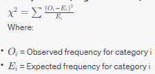
Aynı tedarikçilerden 50'şer parça boyut kontrolünden geçmiş olsun:| Tedarikçi | Uygun | Uygun değil |
|---|---|---|
| A | 46 | 4 |
| B | 37 | 13 |
z-testi: NORM.S.DAĞ
Hurda oranı yıllardır %4 olan bir süreçte yeni bir partinin 800 parçasından 20'si (%2,5) hatalı çıkmış olsun:
Kod:
z = (0,025 − 0,04) / √(0,04 × 0,96 / 800) = −0,015 / 0,00693 = −2,165
p = 2 × (1 − Φ(|z|))  →  =2*(1-NORM.S.DAĞ(MUTLAK(-2,165);DOĞRU))   → 0,0304
İngilizce Excel: =2*(1-NORM.S.DIST(ABS(-2.165),TRUE))7. Tek kuyruklu mu, çift kuyruklu mu? α nasıl seçilir?
Örnekte tek kuyruklu p = 0,0139'dur (alternative="greater"), yani çift kuyruklu değerin tam yarısı; yön ters seçilirse (alternative="less") p = 0,986 olur.- Tek kuyruklu test, yön veriye bakmadan önce belirlendiyse ve ters yöndeki bir sonuç "fark yok" ile aynı kararı doğuracaksa savunulabilir; örneğin yeni tedarikçiye yalnızca daha dayanıklıysa geçecekseniz. Veriyi gördükten sonra tek kuyruğa geçmek tipik bir p-hacking örneğidir.
- α = 0,05 bir gelenektir, kural değildir. Yanlış alarmın pahalı olduğu kararlarda (güvenlik açısından kritik bir parçanın tedarikçisini değiştirmek gibi) 0,01 gibi daha sıkı, keşif amaçlı taramalarda daha gevşek bir eşik seçilebilir; önemli olan eşiği analizden önce yazmaktır. α küçüldükçe gerçek bir farkı kaçırma olasılığı (II. tip hata, β) artar; bunu telafi etmenin yolu örneklemi büyütmektir.
- Çift kuyruklu bir t-testinde p ≤ α olması, 1 − α düzeyindeki güven aralığının (α = 0,05 için %95) 0'ı içermemesiyle aynı karardır.
8. Raporlama: etki büyüklüğü ve güven aralığı
P-değeri, farkın ne kadar büyük olduğunu söylemez. Raporda farkı, güven aralığını, etki büyüklüğünü ve p'nin tam değerini birlikte verin:
Kod:
Fark              = 52,0 − 48,0 = 4,0 MPa
%95 GA (Welch)    = 4,0 ± t(0,975; 9,78) × SE = 4,0 ± 2,235 × 1,549 = [0,54; 7,46] MPa
Cohen's d         = 4,0 / sp = 4,0 / √9,25 = 4,0 / 3,041 = 1,315
Hedges' g = d × (1 − 3 / (4·16 − 1)) = 1,315 × 0,952 = 1,252- Cohen's d farkı birleştirilmiş standart sapmaya böler; Hedges' g, d'nin küçük örneklemlerdeki hafif yukarı yönlü yanlılığını düzeltir. Varyanslar belirgin biçimde farklıysa payda tartışmalıdır (iki varyansın ortalamasının karekökü √10 = 3,16 ile d = 1,26); hangisini kullandığınızı yazın. Cohen'in 0,2/0,5/0,8 (küçük/orta/büyük) ölçütleri bağlamın yerini tutmaz: 4 MPa, parçanızın emniyet payını tüketiyorsa önemlidir.
- Güven aralığı en bilgilendirici çıktıdır: veri, yaklaşık 0,5 MPa ile 7,5 MPa arasındaki gerçek farklarla uyumludur. Bu, "A daha dayanıklı" sonucunu destekliyor ama farkın büyüklüğü belirsiz; pahalı bir karardan önce daha fazla numune test edin.
P-değerini tam haliyle yazın (p = 0,028); yalnızca "p < 0,05" yazmak bilgi kaybettirir.Tedarikçi A'nın numuneleri (n = 8, ortalama 52,0 MPa, ss = 4,0), Tedarikçi B'ninkilerden (n = 10, ortalama 48,0 MPa, ss = 2,0) ortalama 4,0 MPa daha yüksek çekme dayanımı gösterdi; Welch t(9,78) = 2,58, p = 0,028, farkın %95 güven aralığı [0,54; 7,46] MPa, Hedges' g = 1,25.
9. Varsayım kontrolleri ve çoklu karşılaştırma düzeltmeleri
t-testinin varsayımları
- Bağımsızlık: En önemli varsayımdır ve hiçbir testle kanıtlanamaz. Aynı baskı işinde, aynı makaradan ya da tablanın aynı bölgesinde basılan numuneler birbirine benzer; bunları bağımsız saymak çoğu zaman p'yi yapay olarak küçültür. Baskı sırasını ve tabla konumunu rastgele dağıtın; ölçümler partilere kümeleniyorsa parti ortalamalarıyla ya da karma modellerle (mixed models) çalışın.
- Normallik: t-testi normallikten orta düzeydeki sapmalara dayanıklıdır; küçük örneklemde nokta grafiği (dot plot) ya da Q-Q grafiğiyle uç değer ve çarpıklık arayın. Shapiro–Wilk testinin p-değerleri burada 0,99 (A) ve 0,72 (B), ama n = 8'de testin gücü çok düşüktür; bu "normallik kanıtlandı" demek değildir.
- Eşit varyans: Welch buna ihtiyaç duymaz. Levene testi, varyanslar arasında dört kat fark olmasına rağmen p = 0,12 verir; Student ile Welch arasındaki seçimi gücü düşük ön testlere bırakmayın, doğrudan Welch kullanın.
Çoklu karşılaştırma: Bonferroni, Holm ve Benjamini–Hochberg
Hepsinde H0'ın doğru olduğu 20 bağımsız testi α = 0,05 ile yaparsanız en az bir yanlış pozitif görme olasılığı 1 − 0,95^20 ≈ %64'tür. Beş baskı ayarını referans ayarla karşılaştırıp şu p-değerlerini bulduğunuzu düşünün: 0,003; 0,012; 0,021; 0,038; 0,300. Kalın değerler α = 0,05'te anlamlıdır:| Sıralı p | Bonferroni | Holm | BH eşiği (k/5 × 0,05) | BH düzeltilmiş p |
|---|---|---|---|---|
| 0,003 | 0,015 | 0,015 | 0,010 | 0,015 |
| 0,012 | 0,060 | 0,048 | 0,020 | 0,030 |
| 0,021 | 0,105 | 0,063 | 0,030 | 0,035 |
| 0,038 | 0,190 | 0,076 | 0,040 | 0,0475 |
| 0,300 | 1,000 | 0,300 | 0,050 | 0,300 |
- Bonferroni her p'yi test sayısıyla çarpar ve aile boyu hata oranını (familywise error rate, FWER), yani en az bir yanlış pozitif olasılığını α ile sınırlar. Temkinlidir: burada yalnızca 1 sonuç anlamlı kalır.
- Holm aynı güvenceyi verir ama hiçbir zaman Bonferroni'den daha az güçlü değildir. Sıralı p'leri α/5, α/4, α/3… ile karşılaştırır ve eşiği aşan ilk değerde durur: 2 sonuç anlamlı kalır.
- Benjamini–Hochberg (BH) yanlış keşif oranını (false discovery rate, FDR), yani reddedilenler içindeki yanlış pozitiflerin beklenen payını kontrol eder. Küçükten büyüğe sıralı listede k. sıradaki p'yi (k/m)·q ile karşılaştırır (m test sayısı, q hedeflenen FDR düzeyi; burada 0,05) ve eşiği karşılayan en büyük k'ye kadar hepsini reddeder; 0,038 ≤ 0,040 olduğundan 4 sonuç anlamlı kalır. Bağımsız ya da pozitif bağımlı testlerde geçerlidir; değilse Benjamini–Yekutieli (fdr_by) kullanın.
Python:
from statsmodels.stats.multitest import multipletests
from scipy import stats

p = [0.003, 0.012, 0.021, 0.038, 0.300]
for yontem in ("bonferroni", "holm", "fdr_bh"):
    red, p_duz, _, _ = multipletests(p, alpha=0.05, method=yontem)
    print(yontem, red, p_duz.round(4))
print(stats.false_discovery_control(p)) # BH, SciPy 1.11 ve sonrası10. Sık yapılan yorum hataları ve ASA 2016 açıklaması
Amerikan İstatistik Derneği (ASA), 2016'da p-değerleri üzerine altı ilkeden oluşan bir açıklama yayımladı (Wasserstein ve Lazar, The American Statistician, 2016); ilkeler ASA'nın duyurusunda listeleniyor. İlk ilkeye göre p-değeri, verinin belirli bir istatistiksel modelle ne kadar uyumsuz olduğunu gösterebilir. Model H0'ı varsayımlarla birlikte içerir; küçük p bu bütünün bir yerinde sorun olduğunu söyler ama nerede olduğunu söylemez. En sık yapılan hatalar:- "p = 0,028, yani H0'ın doğru olma (ya da sonucun şans eseri çıkma) olasılığı %2,8." Yanlış; p, H0 doğru varsayılarak hesaplanır ve bu olasılıkları veremez (ilke 2).
- "p küçük, demek ki fark büyük ya da önemli." Yanlış (ilke 5). Binlerce ölçümde 0,1 MPa'lık önemsiz bir fark da p < 0,001 verebilir.
- "p = 0,06, demek ki fark yok." Kanıtın yokluğu, yokluğun kanıtı değildir; geniş bir güven aralığı "bu veriyle karar verilemez" demektir (ilke 3 ve 6).
- "p = 0,049 ile p = 0,051 bambaşka sonuçlar." Karar için eşik gerekir ama kanıt süreklidir; bu iki değer neredeyse aynı kanıtı taşır (ilke 3).
- Yalnızca anlamlı çıkan analizleri raporlamak. Kaç test yapıldığı, hangi verilerin dışlandığı ve neyin önceden planlandığı yazılmadıkça p-değerleri yorumlanamaz (ilke 4).
- "1 − p, sonucun tekrarlanma olasılığıdır." Yanlış; 1 − p ne tekrarlanma olasılığıdır ne de H1'in doğru olma olasılığı.
Sık sorulan sorular
Yazılım p = 0,000 gösteriyor, ne yazmalıyım?P-değeri hiçbir zaman tam olarak sıfır olmaz; gördüğünüz değer yuvarlanmıştır. "p < 0,001" yazın ve etki büyüklüğünü ekleyin.
Kaç numune gerekir?
Bunu güç analizi (power analysis) söyler: statsmodels.stats.power.TTestIndPower().solve_power(effect_size=0.8, alpha=0.05, power=0.8) iki bağımsız grup için grup başına yaklaşık 26 gözlem verir; d = 0,5 için bu sayı 64'tür. Beklenen etkiyi önceki verilerden ya da pratikte önemli sayacağınız en küçük farktan tahmin edin.
Welch mi, Student t-testi mi?
Varsayılan olarak Welch. Varyanslar ve grup büyüklükleri benzerse iki test neredeyse aynı sonucu verir; farklıysa Welch güvenilir kalırken Student yanıltabilir.
Excel ile Python farklı p veriyor, hangisi doğru?
Genellikle ikisi de kendi ayarlarına göre doğrudur. T.TEST'in kuyruk ve tür bağımsız değişkenlerini SciPy'daki equal_var ve alternative ayarlarıyla karşılaştırın. Ki-karede fark genellikle Yates düzeltmesinden, Çözümleyici Araç Takımı'nda ise yuvarlanan df'den gelir.
Makine öğrenmesi modellerini p-değeriyle karşılaştırabilir miyim?
Dikkatle. Aynı çapraz doğrulama katlarından (fold) gelen skorlar eşleştirilmiştir ve eğitim kümeleri örtüştüğü için bağımsız değildir; basit bir eşleştirilmiş t-testi p'yi olduğundan küçük gösterebilir. Ayrıntılar için Makine Öğrenmesinde P-Value yazımıza bakın.
Sonuç ve sonraki adımlar
P-değerini hesaplamak birkaç satırlık iş; asıl emek doğru testi seçmek, varsayımları dürüstçe kontrol etmek ve sonucu bağlamıyla raporlamaktır. Örnek veride elle, Python'da ve Excel'de aynı sonuca ulaştık: Welch t(9,78) = 2,58, p = 0,028, fark 4,0 MPa, %95 GA [0,54; 7,46] MPa.- Testi, kuyruk yönünü ve α'yı veri toplanmadan önce yazın.
- Bağımsız iki grup için varsayılan olarak Welch kullanın: SciPy'da equal_var=False, Excel'de T.TEST tür 3.
- Farkı, güven aralığını, etki büyüklüğünü ve p'nin tam değerini birlikte raporlayın; birden çok test yaptıysanız Holm veya BH uygulayın.
- Bir sonraki deneyin numune sayısını güç analiziyle planlayın.
The short answer to "how do I calculate a p-value?": choose the test that fits your data, compute its test statistic (t, z, χ² or F), then take the probability of a statistic at least that extreme under the null hypothesis from that statistic's distribution. For two independent groups, software does all three steps in one call: stats.ttest_ind(a, b, equal_var=False) in Python or =T.TEST(range1,range2,2,3) in Excel. This guide works one small dataset through by hand, in Python and in Excel or Google Sheets, and uses the same example to cover test choice, one- versus two-tailed tests, reporting, assumptions, multiple comparisons and the usual misreadings. Every number was checked with SciPy and statsmodels.
1. What a p-value is: intuition and the correct definition
Every hypothesis test starts from one question: if there were really no difference, how often would random sampling alone produce a difference at least this large? The "no difference" assumption is the null hypothesis (H0); the claim being tested is the alternative hypothesis (H1).Definition: the p-value is the probability of getting a test statistic (t, z, χ² or F) at least as extreme as the one observed, assuming H0 is true and the test's assumptions (independent observations, a suitable distributional model) hold. A small p says the data fit poorly with the model "H0 plus assumptions", and nothing more.
- Significance level (α): the threshold fixed before looking at the data; reject H0 when p ≤ α. α is the probability of rejecting a true H0 (a Type I error).
- Degrees of freedom (df): the parameter that sets the shape of the t, χ² and F distributions; roughly, how much independent information went into the variance estimate. The smaller the df, the heavier the tails of the t distribution.
- One- and two-tailed: whether p comes from one end of the distribution or from both.
2. The worked dataset: filament from two suppliers
A workshop prints tensile test bars from PLA filament bought from two suppliers, with identical settings and a randomized print order, and measures tensile strength in MPa. The numbers are invented for teaching.| Group | Measurements (MPa) | n | Mean | Standard deviation |
|---|---|---|---|---|
| Supplier A | 53, 45, 55, 50, 58, 52, 49, 54 | 8 | 52.0 | 4.0 |
| Supplier B | 47, 50, 46, 48, 51, 45, 49, 48, 50, 46 | 10 | 48.0 | 2.0 |
Hypotheses: H0: μA = μB, H1: μA ≠ μB (two-tailed), with α = 0.05 fixed before the analysis. Group A is both smaller and noisier, and that detail will move the result noticeably.
3. Choosing the test: a decision table
The data type (measurements or counts), the number of groups and whether observations are paired decide the test.| Question and data | Parametric test | Non-parametric alternative | Python |
|---|---|---|---|
| Does one group's mean differ from a target (e.g. 50 MPa)? | One-sample t-test | Wilcoxon signed-rank test | stats.ttest_1samp |
| Do two independent groups differ in mean? | Welch t-test (Student if equal variances are assumed) | Mann–Whitney U | stats.ttest_ind(a, b, equal_var=False) |
| Before/after measurements on the same parts | Paired t-test | Wilcoxon signed-rank test | stats.ttest_rel |
| Three or more independent groups | One-way ANOVA plus a post-hoc test such as Tukey's HSD | Kruskal–Wallis | stats.f_oneway; for unequal variances statsmodels anova_oneway(use_var="unequal") |
| Two categorical variables (counts) | Chi-square test of independence | Fisher's exact test (small expected counts) | stats.chi2_contingency, stats.fisher_exact |
| Population SD genuinely known, or a proportion from a large sample | z-test | Exact binomial test | stats.binomtest, statsmodels proportions_ztest |
Two common mistakes. First, the z-test is not "the test for n > 30": if the standard deviation is estimated from the sample, the right reference distribution is t, which approaches the normal as n grows anyway. Run statsmodels' ztest(a, b) on our data and you get p ≈ 0.006, one fifth of the correct Welch result (0.028). Second, Mann–Whitney U does not compare means; it tests whether values from one group tend to be larger than values from the other, and reading it as a test of medians is only valid when both distributions have the same shape.
4. By hand: t statistic, degrees of freedom and p
Two independent groups with clearly different spreads call for Welch's t-test.Step 1: means and variances
Kod:
A: sum = 416, n = 8   →  mean = 52.0
   deviations from the mean: 1, -7, 3, -2, 6, 0, -3, 2
   sum of squares = 1+49+9+4+36+0+9+4 = 112  →  s² = 112/7 = 16.0  (s = 4.0)

B: sum = 480, n = 10  →  mean = 48.0
   deviations from the mean: -1, 2, -2, 0, 3, -3, 1, 0, 2, -2
sum of squares = 1+4+4+0+9+9+1+0+4+4 = 36 → s² = 36/9 = 4.0 (s = 2.0)Step 2: standard error and t
Kod:
SE = √(sA²/nA + sB²/nB) = √(16/8 + 4/10) = √(2.0 + 0.4) = √2.4 = 1.549
t  = (52.0 − 48.0) / 1.549 = 2.582
Step 3: Welch–Satterthwaite degrees of freedom
Kod:
df = (sA²/nA + sB²/nB)² / [ (sA²/nA)²/(nA−1) + (sB²/nB)²/(nB−1) ]
   = 2.4² / [ 2.0²/7 + 0.4²/9 ]
= 5.76 / (0.5714 + 0.0178) = 5.76 / 0.5892 = 9.78Step 4: from t to a two-tailed p
The p-value is the area in both tails of t(9.78) beyond ±2.582: p = 2 × P(T ≥ 2.582). By hand you bracket it with a t table, rounding a fractional df down to stay conservative:
Kod:
two-tailed critical values for df = 9:
  p = 0.05  →  2.262
  p = 0.02  →  2.821
2.262 < 2.582 < 2.821   →   0.02 < p < 0.05
Kod:
t² = 16 / 2.4 = 6.667
x  = df / (df + t²) = 9.776 / (9.776 + 6.667) = 0.5945
p = I_x(df/2, 1/2) = I_0.5945(4.888, 0.5) = 0.0278For comparison: Student's t-test
Student's test assumes equal variances and pools them: sp² = (7·16 + 9·4)/16 = 9.25, SE = √(9.25 · (1/8 + 1/10)) = 1.443, t = 2.773, df = 16, p = 0.0136. That is about half of Welch's p, because pooling gives too much weight to the larger, less variable group B, hides A's spread and shrinks the standard error. Had the larger group been the noisier one, Student's test would have erred the other way and been too conservative. Using the normal distribution instead of t would give p ≈ 0.0098: ignoring the heavy tails at small df cuts p to about a third.5. In Python: SciPy and statsmodels
Python:
import numpy as np
from scipy import stats

a = np.array([53, 45, 55, 50, 58, 52, 49, 54])          # supplier A
b = np.array([47, 50, 46, 48, 51, 45, 49, 48, 50, 46])  # supplier B

welch = stats.ttest_ind(a, b, equal_var=False)
print(welch.statistic, welch.df, welch.pvalue)   # 2.582  9.776  0.0278
print(welch.confidence_interval(0.95))           # low=0.537, high=7.463

student = stats.ttest_ind(a, b)                  # default: equal_var=True
print(student.statistic, student.df, student.pvalue)   # 2.773  16.0  0.0136

# the p-value straight from the t distribution
t, df = welch.statistic, welch.df
print(2 * stats.t.sf(abs(t), df))   # 0.0278 (two-tailed)
print(stats.t.sf(t, df))            # 0.0139 (one-tailed, H1: A > B)
Python:
from statsmodels.stats.weightstats import ttest_ind, CompareMeans, DescrStatsW

t, p, df = ttest_ind(a, b, usevar="unequal")       # 2.582, 0.0278, 9.776
cm = CompareMeans(DescrStatsW(a), DescrStatsW(b))
print(cm.tconfint_diff(usevar="unequal"))          # (0.537, 7.463)
6. In Excel and Google Sheets
Put group A in A2:A9 and group B in B2:B11. In English-language Excel:
Kod:
Welch p, two-tailed          =T.TEST(A2:A9,B2:B11,2,3)               → 0.0278
Student p                    =T.TEST(A2:A9,B2:B11,2,2)               → 0.0136
Welch p, one-tailed          =T.TEST(A2:A9,B2:B11,1,3)               → 0.0139
Welch t                      =(AVERAGE(A2:A9)-AVERAGE(B2:B11))/SQRT(VAR.S(A2:A9)/COUNT(A2:A9)+VAR.S(B2:B11)/COUNT(B2:B11))   → 2.582
p from Student t (df = 16)   =T.DIST.2T(2.773,16)                    → 0.0136
p from Welch t (df = 9.776) =BETA.DIST(9.776/(9.776+2.582^2),9.776/2,0.5,TRUE) → 0.0278- Fractional df: T.TEST with type 3 uses Welch's df unrounded, while the Analysis ToolPak's unequal-variance t-test tool rounds df to an integer, so the last digits of p can differ. Microsoft documents T.DIST.2T's df argument as an integer (and T.INV.2T explicitly truncates a fractional df), so for a fractional df use T.TEST or the BETA.DIST formula. Truncating df to 9 gives p = 0.0296.
- Localized Excel: function names are translated, and where the decimal mark is a comma (Turkish, German and many other locales) arguments are separated with semicolons, following the operating system's regional settings. In Turkish Excel the Welch test is =T.TEST(A2:A9;B2:B11;2;3), and T.DIST.2T, CHISQ.TEST, NORM.S.DIST and BETA.DIST become T.DAĞ.2K, KİKARE.TEST, NORM.S.DAĞ and BETA.DAĞ.
- Google Sheets: offers T.TEST, T.DIST.2T, CHISQ.TEST and NORM.S.DIST with the same type codes, and separators follow the file's locale (File > Settings). In the same dialog, the "Always use English function names" option decides whether an account set to Turkish or another supported language sees English or localized function names. Google's T.TEST help page asks for both ranges to have the same number of data points, so with unequal group sizes cross-check the result against SciPy. The BETA.DIST that Google documents has no cumulative argument.
Chi-square with CHISQ.TEST
Suppose 50 parts from each supplier went through dimensional inspection:| Supplier | Pass | Fail |
|---|---|---|
| A | 46 | 4 |
| B | 37 | 13 |
z-test with NORM.S.DIST
Say a process has run at a 4% scrap rate for years and a new batch shows 20 defective parts out of 800 (2.5%):
Kod:
z = (0.025 − 0.04) / √(0.04 × 0.96 / 800) = −0.015 / 0.00693 = −2.165
p = 2 × (1 − Φ(|z|))  →  =2*(1-NORM.S.DIST(ABS(-2.165),TRUE))   → 0.0304
Turkish Excel: =2*(1-NORM.S.DAĞ(MUTLAK(-2,165);DOĞRU))7. One-tailed or two-tailed, and how to choose α
For our data the one-tailed p is 0.0139 (alternative="greater"), exactly half the two-tailed value; pick the wrong direction (alternative="less") and p becomes 0.986.- A one-tailed test is defensible only if the direction was fixed before seeing the data and a result in the opposite direction would lead to the same decision as "no difference", for example when you will switch suppliers only if the new one is stronger. Switching to one tail after seeing the data is a textbook case of p-hacking.
- α = 0.05 is a convention, not a law. Where a false alarm is expensive (changing the supplier of a safety-critical part), use a stricter threshold such as 0.01; for exploratory screening a looser one can be acceptable. What matters is writing it down before the analysis. Lowering α raises the chance of missing a real effect (a Type II error, β), and the way to pay for that is a larger sample.
- For a two-tailed t-test, p ≤ α is the same decision as the 1 − α confidence interval (95% for α = 0.05) excluding zero.
8. Reporting: effect size and confidence interval
A p-value says nothing about how big the difference is. Report the difference with its confidence interval, an effect size and the exact p together:
Kod:
Difference        = 52.0 − 48.0 = 4.0 MPa
95% CI (Welch)    = 4.0 ± t(0.975; 9.78) × SE = 4.0 ± 2.235 × 1.549 = [0.54, 7.46] MPa
Cohen's d         = 4.0 / sp = 4.0 / √9.25 = 4.0 / 3.041 = 1.315
Hedges' g = d × (1 − 3 / (4·16 − 1)) = 1.315 × 0.952 = 1.252- Cohen's d divides the difference by the pooled standard deviation; Hedges' g corrects its slight upward bias in small samples. When variances clearly differ, the denominator is debatable (the square root of the average variance, √10 = 3.16, gives d = 1.26), so say which one you used. Cohen's 0.2/0.5/0.8 (small/medium/large) benchmarks are no substitute for context: 4 MPa matters if it eats into your part's safety margin.
- The confidence interval is the most informative output: the data are compatible with a true difference anywhere from about 0.5 MPa to 7.5 MPa. That supports "A is stronger", but the size of the gap is uncertain; test more bars before a costly decision.
Report p exactly (p = 0.028); writing only "p < 0.05" throws information away.Bars from supplier A (n = 8, mean 52.0 MPa, SD 4.0) had a mean tensile strength 4.0 MPa higher than bars from supplier B (n = 10, mean 48.0 MPa, SD 2.0); Welch t(9.78) = 2.58, p = 0.028, 95% CI for the difference [0.54, 7.46] MPa, Hedges' g = 1.25.
9. Assumption checks and multiple-comparison corrections
Assumptions of the t-test
- Independence: the most important assumption, and no test can confirm it. Bars printed in the same job, from the same spool or in the same corner of the bed resemble each other; treating them as independent usually makes p artificially small. Randomize print order and bed position, and if measurements cluster by batch, analyse batch means or use mixed models.
- Normality: the t-test tolerates moderate departures from normality; with small samples, look for outliers and strong skew in a dot plot or Q-Q plot. Shapiro–Wilk p-values here are 0.99 (A) and 0.72 (B), but with n = 8 the test has very little power, so this is not proof of normality.
- Equal variances: Welch's test does not need them. Levene's test returns p = 0.12 here despite a fourfold variance ratio, so do not let weak pre-tests choose between Student and Welch; use Welch by default.
Multiple comparisons: Bonferroni, Holm and Benjamini–Hochberg
If you run 20 independent tests at α = 0.05 and every H0 is true, the chance of at least one false positive is 1 − 0.95^20 ≈ 64%. Suppose you compared five print settings against a reference and got p = 0.003, 0.012, 0.021, 0.038 and 0.300. Bold values are significant at α = 0.05:| Sorted p | Bonferroni | Holm | BH threshold (k/5 × 0.05) | BH-adjusted p |
|---|---|---|---|---|
| 0.003 | 0.015 | 0.015 | 0.010 | 0.015 |
| 0.012 | 0.060 | 0.048 | 0.020 | 0.030 |
| 0.021 | 0.105 | 0.063 | 0.030 | 0.035 |
| 0.038 | 0.190 | 0.076 | 0.040 | 0.0475 |
| 0.300 | 1.000 | 0.300 | 0.050 | 0.300 |
- Bonferroni multiplies each p by the number of tests and caps the familywise error rate (FWER), the chance of any false positive in the family, at α. It is conservative: 1 result survives.
- Holm gives the same guarantee and is never less powerful than Bonferroni. It compares the sorted p-values with α/5, α/4, α/3 and so on, stopping at the first p that misses its threshold: 2 results survive.
- Benjamini–Hochberg (BH) controls the false discovery rate (FDR), the expected share of false positives among the rejected hypotheses. It compares the k-th smallest p with (k/m)·q, where m is the number of tests and q the target FDR (0.05 here), and rejects everything up to the largest k that passes; because 0.038 ≤ 0.040, 4 results survive. It is valid for independent or positively dependent tests; otherwise use Benjamini–Yekutieli (fdr_by).
Python:
from statsmodels.stats.multitest import multipletests
from scipy import stats

p = [0.003, 0.012, 0.021, 0.038, 0.300]
for method in ("bonferroni", "holm", "fdr_bh"):
    reject, p_adj, _, _ = multipletests(p, alpha=0.05, method=method)
    print(method, reject, p_adj.round(4))
print(stats.false_discovery_control(p)) # BH, SciPy 1.11+10. Common misinterpretations and the ASA 2016 statement
In 2016 the American Statistical Association published a statement on p-values built around six principles (Wasserstein and Lazar, The American Statistician, 2016); the principles are listed in the ASA's announcement. The first says a p-value can indicate how incompatible the data are with a specified statistical model. That model bundles H0 with the assumptions, so a small p says something in the bundle is off, not which part. The most common misreadings:- "p = 0.028, so there is a 2.8% chance that H0 is true (or that the result is a fluke)." Wrong. p is computed assuming H0 is true and cannot give either probability (principle 2).
- "p is small, so the difference is large or important." Wrong (principle 5). With thousands of measurements, a trivial 0.1 MPa gap can produce p < 0.001.
- "p = 0.06, so there is no difference." Absence of evidence is not evidence of absence; a wide confidence interval means "these data cannot decide" (principles 3 and 6).
- "p = 0.049 and p = 0.051 are completely different results." A decision rule needs a threshold, but evidence is continuous; those two values carry almost the same evidence (principle 3).
- Reporting only the analyses that came out significant. p-values cannot be interpreted without knowing how many tests were run, which data were excluded and what was planned in advance (principle 4).
- "1 − p is the probability that the result will replicate." Wrong; 1 − p is neither the replication probability nor the probability that H1 is true.
FAQ
My software shows p = 0.000. What do I report?A p-value is never exactly zero; the display is rounding. Report "p < 0.001" and add the effect size.
How many samples do I need?
A power analysis answers that: statsmodels.stats.power.TTestIndPower().solve_power(effect_size=0.8, alpha=0.05, power=0.8) gives about 26 observations per group for two independent groups, and 64 for d = 0.5. Estimate the expected effect from earlier data or from the smallest difference that would matter in practice.
Welch or Student?
Welch by default. With similar variances and group sizes the two give nearly the same answer; when they differ, Welch stays reliable and Student can mislead.
Excel and Python give different p-values. Which one is right?
Usually both, each for its own settings. Compare T.TEST's tails and type arguments with SciPy's equal_var and alternative settings. For chi-square the gap usually comes from the Yates correction; with the Analysis ToolPak, from the rounded df.
Can I compare machine learning models with a p-value?
Carefully. Scores from the same cross-validation folds are paired, and because the training sets overlap they are not independent, so a plain paired t-test can make p look smaller than it should be. Our p-value in machine learning thread covers the pitfalls in feature selection and model comparison.
Conclusion and next steps
Computing a p-value takes a few lines; the real work is choosing the right test, checking assumptions honestly and reporting the result in context. By hand, in Python and in Excel, the worked example gave the same answer: Welch t(9.78) = 2.58, p = 0.028, a 4.0 MPa difference with a 95% CI of [0.54, 7.46] MPa.- Write down the test, the tail direction and α before collecting data.
- Use Welch by default for two independent groups: equal_var=False in SciPy, type 3 in T.TEST.
- Report the difference, its confidence interval, an effect size and the exact p together; if you ran several tests, apply Holm or BH.
- Plan the sample size of the next experiment with a power analysis.
Ekler
Son düzenleyen:


